Background

The median voter theorem stipulates that “no alternative can beat the one preferred by the median voter in pair-wise majority rule elections if the number of voters is odd, voter preferences are single-peaked over a single-policy dimension, and voters vote sincerely.” (Clark et al 429). Anthony Downs showed that this results in both parties converging to the position of the median voter, at which point they are at a Nash equilibrium (Clark et al 430).

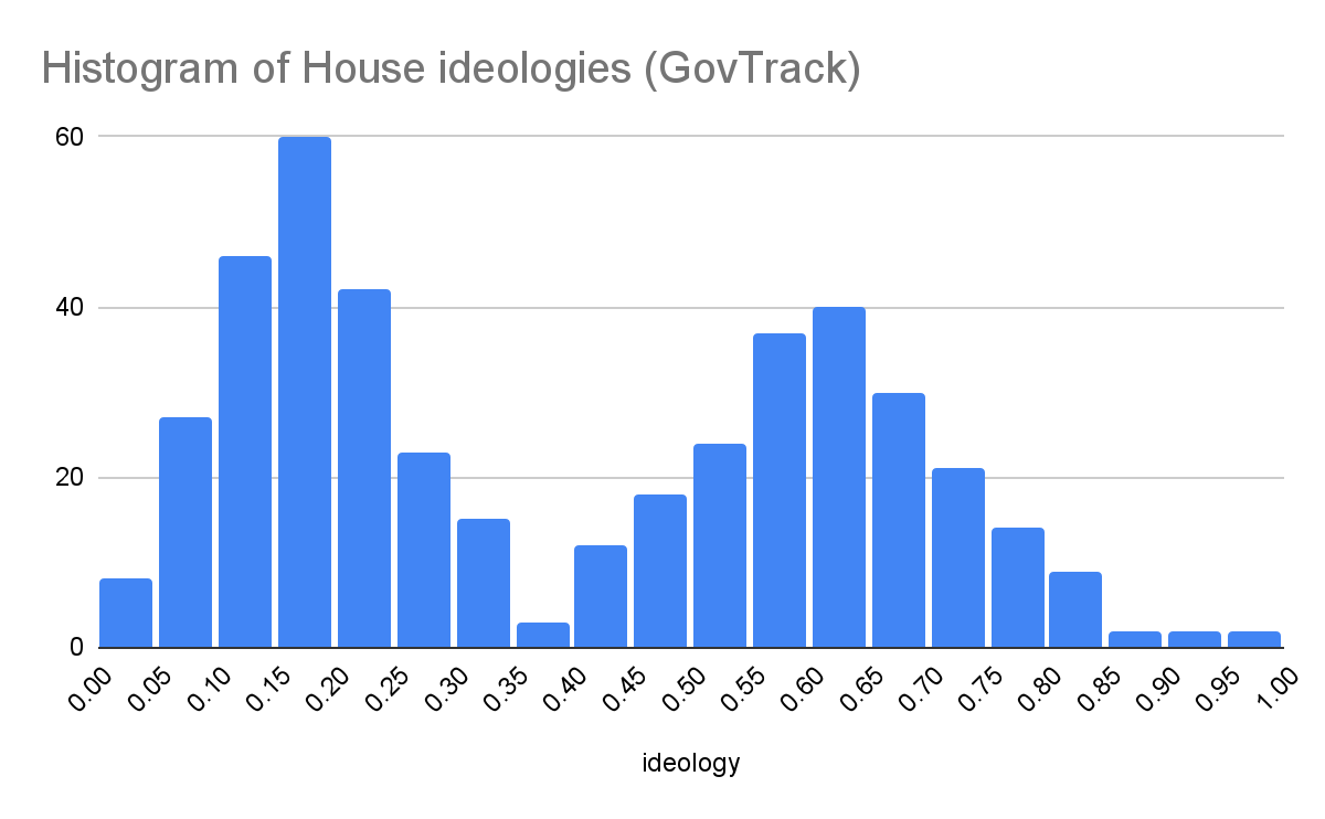
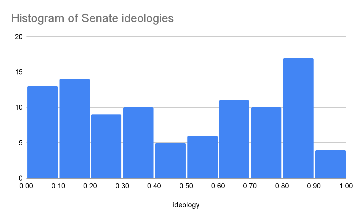
However, this is not what we see in the real world. Focusing on the United States, both national politicians and the American public have been becoming more polarized for decades (DeSilver; Pew Research Center). But while the House and Senate are bimodal in their ideological distributions (GovTrack), the American public is unimodal (Pew Research Center), which implies that national politicians are not simply reflecting the ideologies of voters but have adapted a strategy away from the median voter.

I aim to show that by treating voting as a cost-benefit analysis with the ability to abstain, ideological difference in a two-party system with a normal distribution of ideologies (like the United States) in the voting population can be a party system at equilibrium.

Model

Ideologies will be values between 0 to 100, where 0 is the most left-wing ideology, while 100 is the most right-wing ideology. Voters, the two candidates, and the status quo will each be assigned an ideology.

The voter will have three pure strategies: vote for candidate A, vote for candidate B, or abstain from voting. If the voter votes in a way where candidate A wins, the payoff will be calculated by subtracting the difference between candidate A's ideology and the voter's ideology from the difference between the status quo and the voter's ideology, or in other words, how far the ideology score of reality will move towards the voter's preferred ideology if candidate A wins. If the voter votes in a way where candidate B wins, it follows the same calculations, but with candidate B's ideology score. If the voter doesn't abstain — that is, they vote for either A or B — they will incur a cost of going out to vote. We will also assume that if the votes are tied, the winner will be randomly decided, with each candidate having a 50% chance of winning.

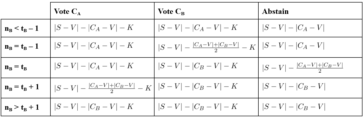
There are five possible conditions under which someone can vote, depending on if and how their vote alone decides the election. The payoffs are laid out in the following table. Let n_B be the number of voters for candidate B, and t_B be the number of voters candidate B needs to win (their tipping point). Let S equal the ideology of the status quo, V equal the voter's ideology, C_A and C_B be the ideologies of candidates A and B respectively, and K equal the cost of voting (expressed as a positive number).^[1]

For simplicity, the model will only use the payoffs for n_B = t_B, or equivalently, where the voter acts as if all other voters are tied and they are the deciding vote. With this condition, for a voter to vote for candidate A,

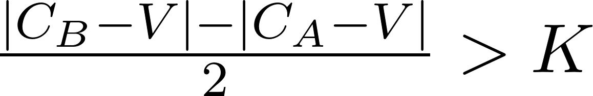
This shows that, according to these payoffs and conditions, one's rational voting behavior does not depend on the status quo.

To determine equilibrium ideological positions for candidates A and B, simulated elections with 3001 normally distributed voters acting according to these payoffs were conducted in the programming language R.

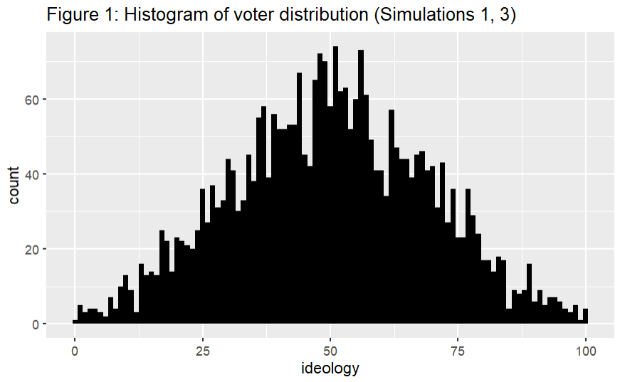
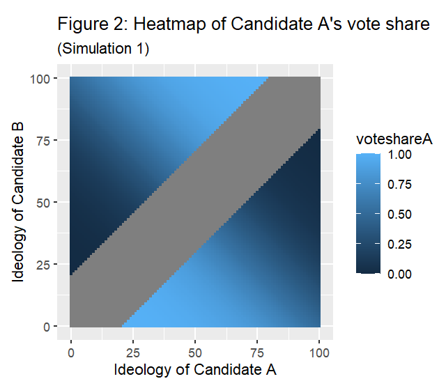
Simulation 1 assigned to voters ideological scores between 0 and 100 (to 3 decimal places), according to a normal distribution^[2] with a mean of 50 and standard deviation of 20 (see distribution in figure 1). This reflects the distribution of voters circa 1995. A cost of 10.4 was assigned.^[3] An election was conducted for each possible pairing of integer ideological scores ranging from 0 to 100 for both candidates: a total of 10,201 elections. Vote shares (out of all votes, not including abstentions) were calculated for each candidate. The vote shares for candidate A are shown in figure 2.^[4] There is a strip of undefined vote shares where all voters abstained, which occurred when half of the difference between candidate A and candidate B's ideologies was less than the cost.

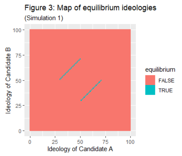
From these results, it was calculated at each pairing of ideological scores whether each candidate had an incentive to deviate; candidate A does not have an incentive to deviate if, given candidate B's ideology, candidate A is at the integer ideology that maximizes their vote share. If neither candidate has an incentive to deviate, they are at Nash equilibrium. Shown in Figure 3, the Nash equilibria occur when the distance between the candidates' ideologies is 21. Nash equilibria only occur with ideologies in the inclusive range of between 30 and 71.

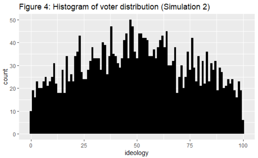
Simulation 2 was identical to Simulation 1, except that it doubled the standard deviation of the voter population, bringing it to 40. This is meant to reflect a more polarized populace, like in modern US politics. However, Simulation 2 had identical Nash equilibria to Simulation 1.

Simulation 3 was also identical to Simulation 1, except that it doubled the cost of voting, bringing it to 20.8. Simulation 3 did have differing Nash equilibria. The Nash equilibria occur when the distance between the candidates' ideologies is 42, and with ideologies in the inclusive range of between 9 and 91.

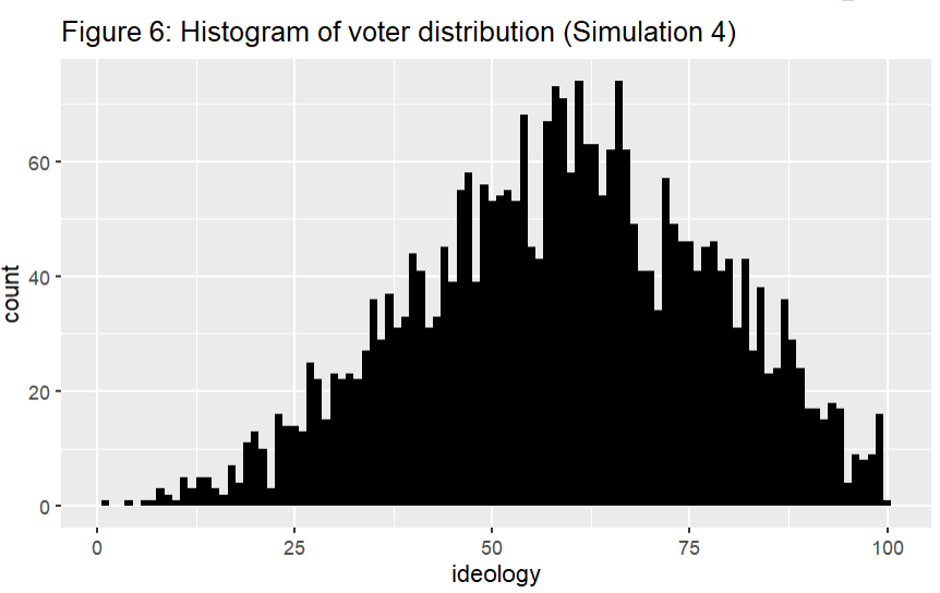
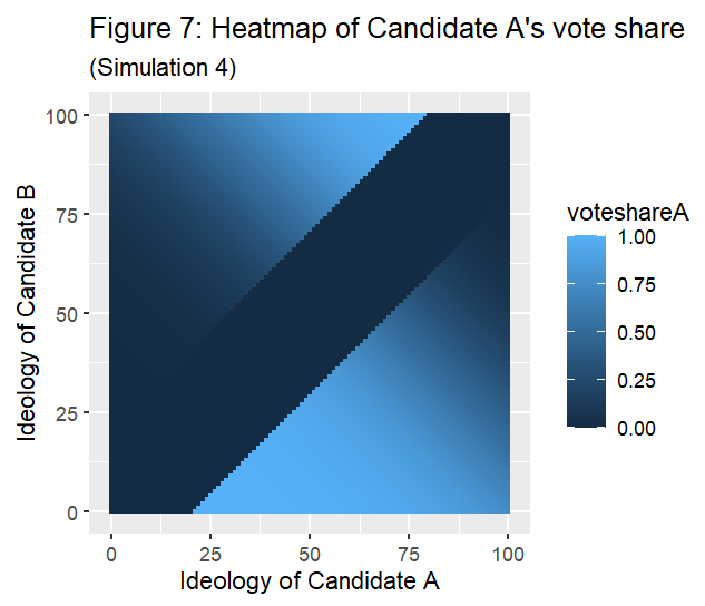
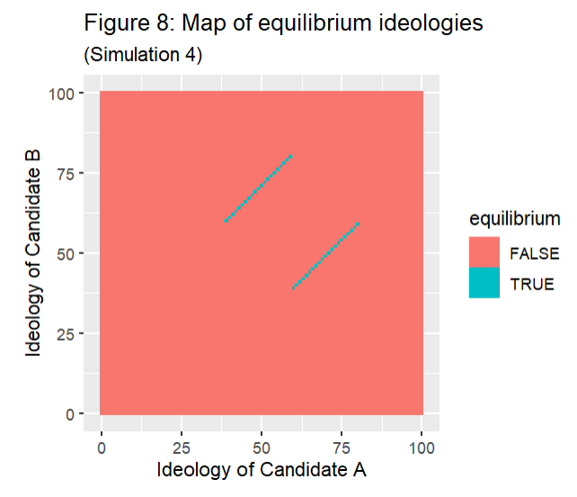
Simulation 4 was also identical to Simulation 1, but the mean of the distribution was changed to 60. The Nash Equilibria again occurred when the distance between the candidates' ideologies was 21, but they occurred with the ideologies in the inclusive range of between 39 and 80.

Discussion

My model demonstrates that, by introducing a cost to voting and by giving voters the ability to abstain from voting, two candidates with ideological differences can be at Nash equilibrium. In fact, with a positive, non-zero cost, there needs to be ideological difference for the candidates to be at equilibrium.

The Nash equilibria occur when the distance between the candidate's ideologies is (the integer above) twice the cost, within the range from (the integer above) the median voter's ideology minus twice the cost to (the integer below) the median voter's ideology plus twice the cost.

I didn't expect the positions of the Nash equilibria — the equilibrium polarization of the candidates — to not depend on the polarization of the voter population, but rather only on the cost of voting (along with the median voter). The rationale makes sense in hindsight: people won't bother to go out to vote if there isn't a substantial difference between the candidates. This potentially suggests that voter suppression is increasing candidate polarization in the United States. Since 2013 — when Shelby County v. Holder eliminated the Justice Department's authority to block changes to state voting laws — there has been a rise in discriminatory voter laws (Bradner). However, these laws target populations that tend to vote for Democrats more than Republicans, which the model doesn't account for with its single cost value.

There are other limitations to the model. In reality, when there are two ideologically similar candidates, we do not see zero votes. This discrepancy could be because there is a level of individual cost unaccounted for in the model, or because a one-dimensional ideological score is unrealistic. Introducing variation to the cost and more dimensions to the ideology scores could remedy this drop-off issue. However, it is unclear whether or not the Nash equilibria will be candidate pairings with ideological difference in a more realistic model where there are still votes (albeit fewer votes) in the range with ideologically similar candidates.

Additionally, the model only uses the payoffs where voters act as if they are the deciding vote. A more comprehensive model could account for imperfect information by weighing the payoffs to account for the probabilities of each condition, although it is unclear what those probabilities should be.

In a way, the model extends the median voter theorem, because the Nash equilibrium values still surround the median voter, but with a distance related to the cost of voting. Additionally, the winner at these equilibria is the candidate closest to the median.